CyRK Performance

CyRK’s C++ backend is highly optimized to solve ODEs using Runge-Kutta methods. It has been tested and benchmarked against the popular SciPy.solve_ivp tool and generally performs much better due to it being typed, compiled, and cache optimized.

There are some considerations regarding performance that users should keep in mind, particularly if they are noticing poorer than anticipated integration times. Most of the conversation here is directed towards cysolve_ivp and CyRK’s C++ backend. However, pysolve_ivp uses the same backend so these considerations still matter, but poor performance is magnified by the overhead that Python imposes.

Tip

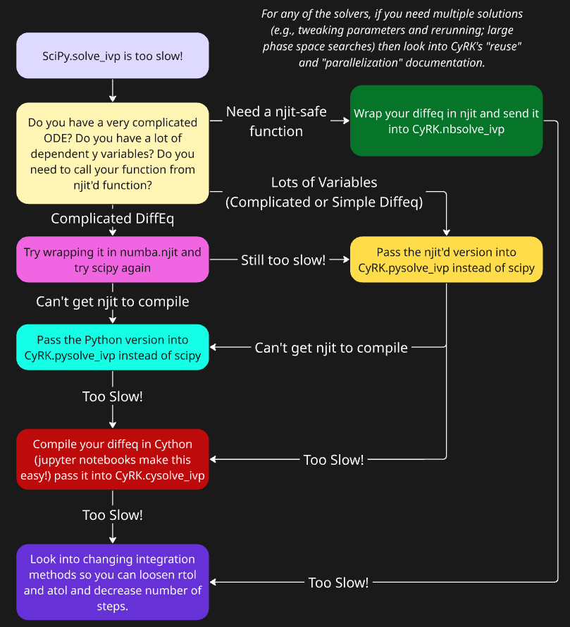
The tl;dr of this section: If you want improved performance follow this decision tree!

Number of Dependent Variables

The size of a ODE system is determined by the number of dependent \(y\) variables (\(N_{y}\)). The more variables, the higher the solver overhead will be as it must loop through all variables several times for each time step. The number of y loops, excluding any in the actual differential equation, is: 4 + 5+/step (RK23); 4 + 8+/step (RK45); 4 + 14+/step (DOP853). Each of the N+/step could be significantly more than the value listed if it takes a while to find a proper step size. Even if it was perfect at predicting step sizes, a 100 step integration would have over 800 \(y\)-loops for the RK45 method.

In addition to these computational considerations, the memory footprint of the solver and the solution structure will increase with the number of y. For double floating point numbers, the \(y\)-specific footprint of the solver is (in Bytes): \(112 N_{y}\) (RK23), \(136 N_{y}\) (RK45), and \(224 N_{y}\) (DOP853). This is just the \(y\)-dependent memory not other overheads (the other overheads are around 1,500 kB). So for RK45, if \(N_{y} = 10,000\), the solver would be over 1 MB. During integration the solution will also be added to at each time step and the data storage grows as \(8*(1+N_{y})\) Bytes/step. If the same 10,000 \(N_{y}\) ODE takes 100 steps to complete, the memory usage will approach 10 MB. While this is a relatively small amount for modern PCs, it can be significant for both RAM limitations if running many solvers in parallel, and cache misses which are a major source of poor performance in CyRK.

Differential Equation Optimization

A critical part of improving performance of any integration is optimizing the problem’s differential equation. The diffeq is called to both determine step error and find the actual derivative at each time step. The diffeq is called at minimum: 3+/step (RK23); 6+/step (RK45); 13+/step (DOP853). Similar to the \(y\)-loops discussed earlier, this number could be much larger if the error is large (or the integration tolerances are small) during a step.

Expect the diffeq to be called 1000s of times for a typical integration. Slow diffeqs quickly become the bottleneck of the integrator. Providing a Cython (or C) compiled or a numba.njit JIT compiled diffeq to CyRK will usually cause orders of magnitude better performance.

Reducing Number of Steps

The prior conversation has focused on the “per step” performance. Reducing the number of steps will always greatly improve overall integration time. There are four factors that affect the number of steps. The first two are generally fixed by the problem with little flexibility: the complexity of the ODE (simpler ODE’s require fewer steps) and the size of the domain of integration (a smaller time domain means less steps). The latter might be helped by using events to cause an early termination based on user-defined criteria. Keep in mind that events carry their own performance overhead so it is better to pick a smaller domain if you can guess it ahead of time.

The last two factors affecting the number of steps, and which are more adjustable, are integration tolerances (rtol and atol) and the integration method (“RK23”, “RK45”, “DOP853”). The integration tolerances directly affect the number of steps because the solver must decrease step size to fit within smaller tolerances. It is important to keep in mind that CyRK allows atol and rtol to be provided as an array, one for each \(y\). This can be helpful if one parameter changes much slower than others (does not need as high a rtol) or is generally much larger than the others (smaller atol). The integration method indirectly affects the number of steps by providing a different level of confidence at a given error level. For example, DOP853 will know much more about the overall ODE at the same error level compared to RK45 (and the same for RK45 compared to RK23). So you can usually loosen the tolerances (make rtol and atol larger) when moving to more complex solver methods (e.g., perhaps you need rtol=1.0e-6 for RK23 to achieve your desired error level but only rtol=1.0e-3 for DOP853 for the same confidence).

As discussed earlier, the more complex methods are much more computationally expensive all else being equal. If you are not able to loosen tolerances then you are better off using a simpler method. The per step cost is always highest for DOP853 > RK45 > RK23. The benefit of DOP853 over RK45 (or RK45 over RK23) is better accuracy with looser tolerances and less steps. Less steps means less computing power. Benchmarking can tell you if that savings outweighs the increased per step cost.

Fewer Steps, Dense Output, and t_eval

Read more about dense outputs and t_eval here.

While decreasing the number of steps will improve performance, it may not produce your desired outcome. If you only care about the solution of an ODE at \(t=t_{end}\), then it is perfect. However, if you want the solution at every \(t_x\) time then you probably are not going to get that since CyRK’s adaptive step solver creates uneven step sizes. This is where the t_eval parameter comes in: Users provide a desired time domain array and CyRK will interpolate the solution to find a value at each provided \(t\) while only taking the minimum necessary “real” steps. Each integration method includes a sophisticated interpolator (these are not simple linear interpolations) so the error at each interpolated step is quite small (depending on the provided rtol and atol).

CyRK also provides a way to store these interpolators to the final solution so that you can perform post-integration “calls” to the solution. For example, say the solution sol to an ODE was found with CyRK with the argument capture_dense=True. After integration if the user wants the solution at a \(t_{new}\) that is within the solution domain but not in the final sol.t array, it can be found using y_new = sol.call(t_new) (the specific syntax varies for the different solvers; see demos).

Keep in mind that using t_eval and especially capture_dense=True carries performance penalties.

CyRK Benchmarks and Discussion

Below is the general benchmark shown else where in CyRK’s documentation and repository. It uses a 2-component ODE that mimics a basic predator-prey model. The different colors represent: Blue = scipy.solve_ivp; Magenta = scipy.solve_ivp using a numba.njit'd diffeq; Cyan = CyRK.pysolve_ivp; Orange = CyRK.pysolve_ivp using a numba.njit'd diffeq; Green = CyRK.nbsolve_ivp; and Red = CyRK.cysolve_ivp. The different symbols indicate different settings that can be turned on or off in the various solvers.

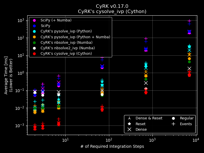
This is a simple diffeq meaning that even the Python version is not terribly slow so numba.njit helps with the speeding up the diffeq, but its not major. This problem is also small with only two dependent \(y\) variables meaning that most of the optimizations in scipy.solve_ivp that utilize numpy ndarray logic is lost. The bulk of the performance comes down to the overhead of the solver, and that is where CyRK.cysolve_ivp really shines. In most cases it beats scipy by a factor of 100x up to 400x.

Many Dependent \(y\) Variables

If we increase the number of dependent variables we start to see CyRK get closer to scipy since scipy is able to lean on numpy’s array math (which is highly optimized). In the example below we utilize a simple diffeq but an ODE system with \(N_{y} = 10,000\) dependent \(y\) variables.

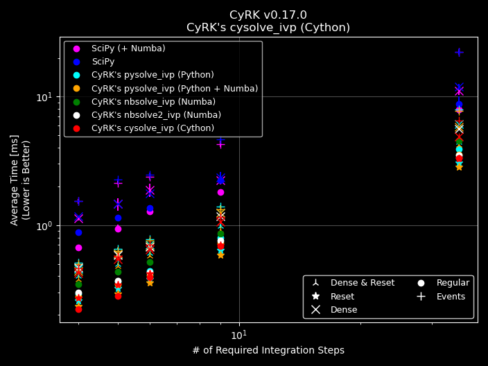
Even though scipy has to contend with the Python overhead, SciPy ends up only being about a factor of 4x slower than CyRK.cysolve_ivp.

Complex DiffEq’s and Many Dependent \(y\) Variables

The prior examples used very simple diffeq’s which run quickly even in Python. In this next example we look at a much more complicated diffeq. It has \(N_{y} = 10,000\) dependent \(y\) variables like the previous example. It also couples them to each other and uses trig functions.

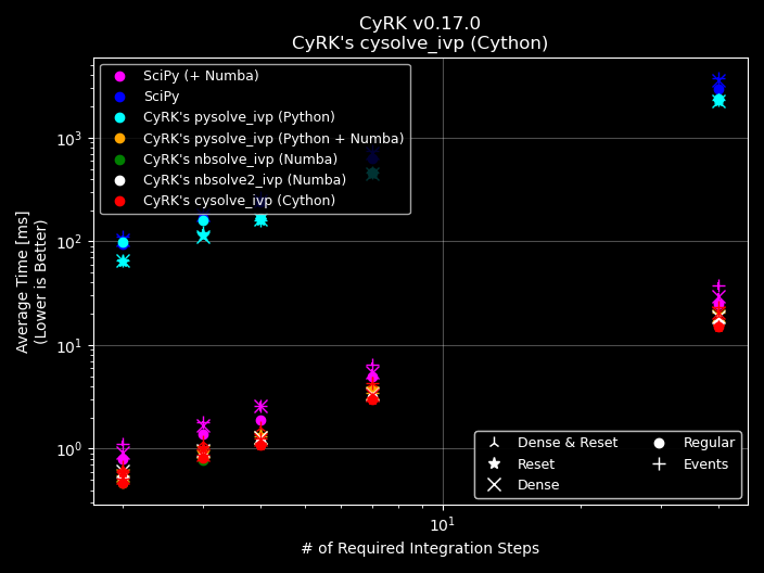
numba.njit is the real champion here. Using a njit’d diffeq with scipy produces results that are only slightly slower than CyRK. The bottleneck here is the complex diffeq and how poorly optimized it is in Python. scipy’s numpy array math is not able to save it from the expense of the diffeq. Even CyRK.pysolve suffers greatly since it to is having to deal with an unoptimized Python diffeq. All of the other solvers do quite well with CyRK.cysolve_ivp slightly eeking out the others (but being around 200x faster than regular scipy). Overall this integration may still be slow even for the faster solvers. If the DiffEq can not be optimized (e.g., maybe we could use taylor expansions on the trig functions or other tricks) then the only tool left is reducing the number of steps, see section above.