Demos and Benchmarks for CyRK’s Solvers
As of CyRK v0.17.0, on a mid-tier desktop the following timings were found:
Function |
Avg. Time [ms] |
|---|---|
SciPy.solve_ivp |
8.240 |
CyRK.nbsolve_ivp |
0.168 |
CyRK.nbsolve2_ivp |
0.073 |
CyRK.pysolve_ivp |
0.315 |
CyRK.cysolve_ivp |
0.036 |
[22]:
import numpy as np
from scipy.integrate import solve_ivp
import matplotlib.pyplot as plt
from numba import njit
plt.style.use('dark_background')

import CyRK
print("CyRK Version:", CyRK.__version__)
from CyRK import nbsolve_ivp, nbsolve2_ivp, nb_diffeq_addr, njit_test_nbsolve_ivp
from CyRK import pysolve_ivp

# Hack the cython magic so that it can set the correct C++ standard.
%load_ext Cython
CyRK Version: 0.17.0
The Cython extension is already loaded. To reload it, use:
  %reload_ext Cython
Hack IPython Magic
In order to make this notebook work across platforms without changes we need to hack the cython cells to include some additional header information. This is done using the script jupyter_cyhack.py file contained in the same directory as these demos. Hopefully it works fine for you, but keep in mind that the hack below is required to get these cells to work. So if you are making your own cythonized notebook you will want to see what headers should be included for your operating system.
[2]:
from Cython.Build import IpythonMagic

from jupyter_cyhack import build_hack

# Get the current cython Ipython parser.
original_cython_parser = IpythonMagic.CythonMagics.cython
# Apply hacks to headers and compile lines.
patched_cython_parser = build_hack(original_cython_parser)
# Patch it in
IpythonMagic.CythonMagics.cython = patched_cython_parser
# Reload
ip = get_ipython()
ip.register_magics(IpythonMagic.CythonMagics)
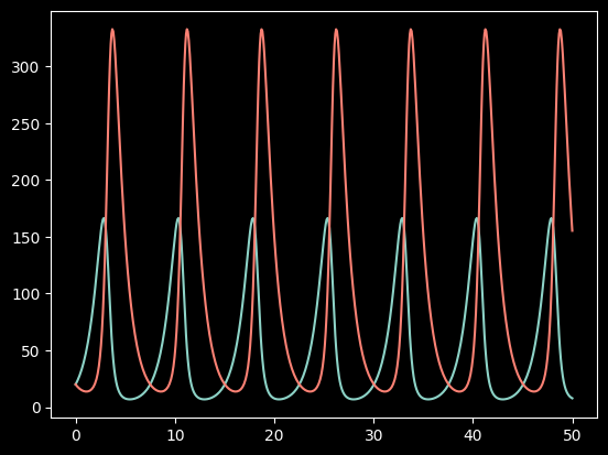
SciPy’s solve_ivp For Comparison
[3]:
def diffeq(t, y):
    dy = np.empty_like(y)
    dy[0] = (1. - 0.01 * y[1]) * y[0]
    dy[1] = (0.02 * y[0] - 1.) * y[1]
    return dy

initial_conds = np.asarray((20., 20.), dtype=np.float64, order='C')
time_span = (0., 50.)
rtol = 1.0e-7
atol = 1.0e-8

result = \
    solve_ivp(diffeq, time_span, initial_conds, method='RK45', rtol=rtol, atol=atol)

print("Was Integration was successful?", result.success)
print(result.message)
fig, ax = plt.subplots()
ax.plot(result.t, result.y[0], c='C0')
ax.plot(result.t, result.y[1], c='C3')
plt.show()
Was Integration was successful? True
The solver successfully reached the end of the integration interval.
[4]:
%timeit solve_ivp(diffeq, time_span, initial_conds, method='RK45', rtol=rtol, atol=atol)
8.24 ms ± 52.4 μs per loop (mean ± std. dev. of 7 runs, 100 loops each)
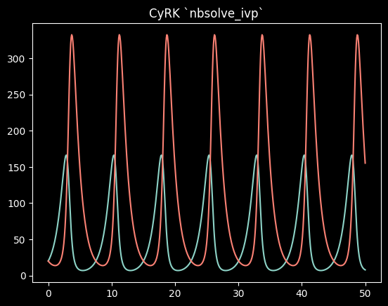
nbsolve_ivpand nbsolve2_ivp Example
[24]:
@njit
def diffeq_nb(t, y):
dy = np.empty_like(y)
dy[0] = (1. - 0.01 * y[1]) * y[0]
dy[1] = (0.02 * y[0] - 1.) * y[1]
return dy
initial_conds = np.asarray((20., 20.), dtype=np.float64, order='C')
time_span = (0., 50.)
rtol = 1.0e-7
atol = 1.0e-8
result = \
nbsolve_ivp(diffeq_nb, time_span, initial_conds, rk_method=1, rtol=rtol, atol=atol)
print("Was Integration was successful?", result.success)
print(result.message)
print("Size of solution: ", result.size)
fig, ax = plt.subplots()
ax.set_title("CyRK `nbsolve_ivp`")
ax.plot(result.t, result.y[0], c='C0')
ax.plot(result.t, result.y[1], c='C3')
plt.show()
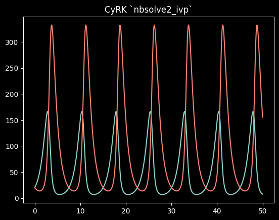
# `nbsolve2_ivp` requires the cfunc address of our function. It also must have the following format
def diffeq_nb2(dy, t, y, args):
dy[0] = (1. - 0.01 * y[1]) * y[0]
dy[1] = (0.02 * y[0] - 1.) * y[1]
diffeq_addr = nb_diffeq_addr(diffeq_nb2)
result = \
nbsolve2_ivp(diffeq_addr, time_span, initial_conds, method='RK45', rtol=rtol, atol=atol)
print("Was Integration was successful?", result.success)
print(result.message)
print("Size of solution: ", result.size)
fig, ax = plt.subplots()
ax.set_title("CyRK `nbsolve2_ivp`")
ax.plot(result.t, result.y[0], c='C0')
ax.plot(result.t, result.y[1], c='C3')
plt.show()
# We must manually free the result from `nbsolve2_ivp`
result.free()
DEPRECATION WARNING! This version of `nbsolve_ivp` will be deprecated in a future release in favor of the current `nbsolve2_ivp` (names will be swapped). These two functions are quite different so please review the documentation at https://cyrk.readthedocs.io/en/latest/Numba.html before upgrading.
IMPORTANT!! Printing this warning is slowing down your integration! Disable it by setting `warnings=False` in `nbsolve_ivp`.
Was Integration was successful? True
Integration completed without issue.
Size of solution:  360
Was Integration was successful? True
Integration completed without issue.
Size of solution:  360
[26]:
%timeit nbsolve_ivp(diffeq_nb, time_span, initial_conds, rk_method=1, rtol=rtol, atol=atol, warnings=False)
168 μs ± 1.93 μs per loop (mean ± std. dev. of 7 runs, 10,000 loops each)
[28]:
%timeit njit_test_nbsolve_ivp(diffeq_addr, time_span, initial_conds, method='RK45', rtol=rtol, atol=atol)
73.1 μs ± 2.02 μs per loop (mean ± std. dev. of 7 runs, 10,000 loops each)
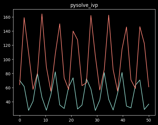
pysolve_ivp Example
[7]:
# Note if using this format, `dy` must be the first argument. Additionally, a special flag must be set to True when calling pysolve_ivp, see below.
def cy_diffeq(dy, t, y):
    dy[0] = (1. - 0.01 * y[1]) * y[0]
    dy[1] = (0.02 * y[0] - 1.) * y[1]

# Since this is pure python we can njit it safely
cy_diffeq = njit(cy_diffeq)

initial_conds = np.asarray((20., 20.), dtype=np.float64, order='C')
time_span = (0., 50.)
rtol = 1.0e-7
atol = 1.0e-8

result = \
    pysolve_ivp(cy_diffeq, time_span, initial_conds, method="RK45", rtol=rtol, atol=atol,
                # Note if you did build a differential equation that has `dy` as the first argument then you must pass the following flag as `True`.
                # You could easily pass the `diffeq_nb` example which returns dy. You would just set this flag to False (and experience a hit to your performance).
                pass_dy_as_arg=True)

print("Was Integration was successful?", result.success)
print(result.message)
print("Size of solution: ", result.size)
fig, ax = plt.subplots()
ax.plot(result.t, result.y[0], c='C0')
ax.plot(result.t, result.y[1], c='C3')
plt.show()
Was Integration was successful? True
Integration completed without issue.
Size of solution:  360

[8]:
%timeit pysolve_ivp(cy_diffeq, time_span, initial_conds, method="RK45", rtol=rtol, atol=atol, pass_dy_as_arg=True)
315 μs ± 8.18 μs per loop (mean ± std. dev. of 7 runs, 1,000 loops each)
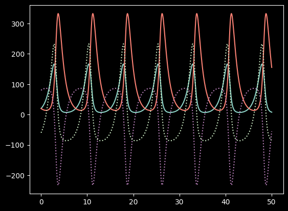
cysolve_ivp Example
[9]:
%%cython --force
# cython: boundscheck=False, wraparound=False, nonecheck=False, cdivision=True, initializedcheck=False
from libcpp.utility cimport move
from libcpp.vector cimport vector

import numpy as np
cimport numpy as np
np.import_array()

# Note the "distutils" and "cython" headers above are functional. They tell cython how to compile the code. In this case we want to use C++ and to turn off several safety checks (which improve performance).

# The cython diffeq is much less flexible than the others described above. It must follow this format, including the type information.
# Currently, CyRK only allows additional arguments to be passed in as a double array pointer (they all must be of type double). Mixed type args will be explored in the future if there is demand for it (make a GitHub issue if you'd like to see this feature!).
# The "noexcept nogil" tells cython that the Python Global Interpretor Lock is not required, and that no exceptions should be raised by the code within this function (both improve performance).
# If you do need the gil for your differential equation then you must use the `cysolve_ivp_gil` function instead of `cysolve_ivp`

# Import the required functions from CyRK
from CyRK cimport cysolve_ivp, DiffeqFuncType, WrapCySolverResult, CySolveOutput, PreEvalFunc

# Note that currently you must provide the "char* args, PreEvalFunc pre_eval_func" as inputs even if they are unused.
# See "Advanced CySolver.md" in the documentation for information about these parameters.
cdef void cython_diffeq(double* dy, double t, double* y, char* args, PreEvalFunc pre_eval_func) noexcept nogil:

    # Unpack args
    # CySolver assumes an arbitrary data type for additional arguments. So we must cast them to the array of
    # doubles that we want to use for this equation
    cdef double* args_as_dbls = <double*>args
    cdef double a = args_as_dbls[0]
    cdef double b = args_as_dbls[1]

    # Build Coeffs
    cdef double coeff_1 = (1. - a * y[1])
    cdef double coeff_2 = (b * y[0] - 1.)

    # Store results
    dy[0] = coeff_1 * y[0]
    dy[1] = coeff_2 * y[1]
    # We can also capture additional output with cysolve_ivp.
    dy[2] = coeff_1
    dy[3] = coeff_2

# Import the required functions from CyRK
from CyRK cimport cysolve_ivp, DiffeqFuncType, WrapCySolverResult, CySolveOutput

# Let's get the integration number for the RK45 method
from CyRK cimport ODEMethod

# Now let's import cysolve_ivp and build a function that runs it. We will not make this function `cdef` like the diffeq was. That way we can run it from python (this is not a requirement. If you want you can do everything within Cython).
# Since this function is not `cdef` we can use Python types for its input. We just need to clean them up and convert them to pure C before we call cysolve_ivp.
def run_cysolver(tuple t_span, double[::1] y0):

    # Cast our diffeq to the accepted format
    cdef DiffeqFuncType diffeq = cython_diffeq

    # Convert the python user input to pure C types
    cdef size_t num_y          = len(y0)
    cdef double t_start        = t_span[0]
    cdef double t_end          = t_span[1]
    cdef vector[double] y0_vec = vector[double](num_y)
    cdef size_t yi
    for yi in range(num_y):
        y0_vec[yi] = y0[yi]

    # Assume constant additional arguments
    # These args are stored in a vector<char>
    cdef vector[char] args_vec = vector[char](2 * sizeof(double)) # Size of vector is size of arg datatype x number of args.

    # Convert to double pointer to more easily populate the vector.
    cdef double* args_as_dbl = <double*>args_vec.data()
    args_as_dbl[0] = 0.01
    args_as_dbl[1] = 0.02
    # Keep in mind these args could be any arbitrary C/C++ structure.

    # Run the integrator!
    cdef CySolveOutput result = cysolve_ivp(
        diffeq,
        t_start,
        t_end,
        y0_vec,
        method = ODEMethod.RK45, # Integration method
        rtol = 1.0e-7,
        atol = 1.0e-8,
        args_vec = args_vec,
        num_extra = 2
    )

    # The CySolveOutput is not accesible via Python. We need to wrap it first
    cdef WrapCySolverResult pysafe_result = WrapCySolverResult()
    pysafe_result.set_cyresult_pointer(move(result))

    return pysafe_result
Content of stdout:
_cython_magic_5a6dd41fee6fb519029f6188c94a11fdc5910c66adad4001cde400fb41db6ae2.cpp
C:\Users\joepr\.ipython\cython\_cython_magic_5a6dd41fee6fb519029f6188c94a11fdc5910c66adad4001cde400fb41db6ae2.cpp(25057): warning C4551: function call missing argument list
C:\Users\joepr\.ipython\cython\_cython_magic_5a6dd41fee6fb519029f6188c94a11fdc5910c66adad4001cde400fb41db6ae2.cpp(25058): warning C4551: function call missing argument list
C:\Users\joepr\.ipython\cython\_cython_magic_5a6dd41fee6fb519029f6188c94a11fdc5910c66adad4001cde400fb41db6ae2.cpp(25181): warning C4551: function call missing argument list
C:\Users\joepr\.ipython\cython\_cython_magic_5a6dd41fee6fb519029f6188c94a11fdc5910c66adad4001cde400fb41db6ae2.cpp(28822): warning C4551: function call missing argument list
C:\Users\joepr\.ipython\cython\_cython_magic_5a6dd41fee6fb519029f6188c94a11fdc5910c66adad4001cde400fb41db6ae2.cpp(28829): warning C4551: function call missing argument list
C:\Users\joepr\.ipython\cython\_cython_magic_5a6dd41fee6fb519029f6188c94a11fdc5910c66adad4001cde400fb41db6ae2.cpp(29187): warning C4551: function call missing argument list
C:\Users\joepr\.ipython\cython\_cython_magic_5a6dd41fee6fb519029f6188c94a11fdc5910c66adad4001cde400fb41db6ae2.cpp(29188): warning C4551: function call missing argument list
   Creating library C:\Users\joepr\.ipython\cython\Users\joepr\.ipython\cython\_cython_magic_5a6dd41fee6fb519029f6188c94a11fdc5910c66adad4001cde400fb41db6ae2.cp312-win_amd64.lib and object C:\Users\joepr\.ipython\cython\Users\joepr\.ipython\cython\_cython_magic_5a6dd41fee6fb519029f6188c94a11fdc5910c66adad4001cde400fb41db6ae2.cp312-win_amd64.exp
Generating code
Finished generating code
[10]:
# Assume we are working in a Jupyter notebook so we don't need to import `run_cysolver` if it was defined in an earlier cell.
# from my_cython_code import run_cysolver

import numpy as np
initial_conds = np.asarray((20., 20.), dtype=np.float64, order='C')
time_span = (0., 50.)

result = run_cysolver(time_span, initial_conds)

print("Was Integration was successful?", result.success)
print(result.message)
print("Size of solution: ", result.size)
import matplotlib.pyplot as plt
fig, ax = plt.subplots()
ax.plot(result.t, result.y[0], c='C0')
ax.plot(result.t, result.y[1], c='C3')

# Can also plot the extra output. They are small for this example so scaling them up by 100
ax.plot(result.t, 100*result.y[2], c='C7', ls=':')
ax.plot(result.t, 100*result.y[3], c='C8', ls=':')
plt.show()
Was Integration was successful? True
Integration completed without issue.
Size of solution:  360
[11]:
%timeit run_cysolver(time_span, initial_conds)
36 μs ± 472 ns per loop (mean ± std. dev. of 7 runs, 10,000 loops each)
Result Structure
Below are the details of the Python-accesible CySolverResult object (called WrapCySolverResult defined in “cysolver_api.pyx”).
[12]:
# First run pysolver to get a result
from numba import njit
import numpy as np
from CyRK import pysolve_ivp

@njit
def cy_diffeq(dy, t, y):
    dy[0] = (1. - 0.01 * y[1]) * y[0]
    dy[1] = (0.02 * y[0] - 1.) * y[1]
initial_conds = np.asarray((20., 20.), dtype=np.float64, order='C')
time_span = (0., 50.)
rtol = 1.0e-7
atol = 1.0e-8
result = pysolve_ivp(cy_diffeq, time_span, initial_conds, method="RK45", rtol=rtol, atol=atol, pass_dy_as_arg=True, dense_output=True)

# Basic information
print("result.success =           ", result.success)
print("result.message =           ", result.message)
print("result.integration_method =", result.integration_method)
print("result.steps_taken =       ", result.steps_taken)
print("result.num_y =             ", result.num_y)
print("result.status =            ", result.status)
print("result.status_message =    ", result.status_message)
print()

# More detailed information (helpful for debugging)
result.print_diagnostics()
print()

# Data arrays (just printing the first few)
print("result.t[:5]    =", result.t[:5])
print("result.y[0, :5] =", result.y[0, :5])
print("result.y[1, :5] =", result.y[1, :5])
print()

# Since we captured dense outputs, we can make calls to the diffeq solution
new_t = 25.5
print("Solution at new_t:", result.call(new_t))
new_t_arr = np.linspace(20.0, 22.0, 5)
y_at_t_arr = result.call_vectorize(new_t_arr)
print("Solution at new_t_arr:\n\ty0=", y_at_t_arr[0,:], "\n\ty1=", y_at_t_arr[1,:])
# Can also directly call the result with either a float or an array
print("Direct call new_t:", result(new_t))
result.success =            True
result.message =            Integration completed without issue.
result.integration_method = Explicit Runge-Kutta method of order 5(4)
result.steps_taken =        359
result.num_y =              2
result.status =             1
result.status_message =     Integration completed without issue.

----------------------------------------------------
CyRK v0.17.0 - WrapCySolverResult Diagnostic.
----------------------------------------------------
# of y:             2.
# of dy:            2.
# of events:        0.
Success:            True.
Error Code:         1.
Status:             Integration completed without issue..
Size:               360.
Steps Taken:        359.
Event Termination:  False.
Integrator Message:
        Integration completed without issue.

----------------- CySolverResult -------------------
Capture Extra:          False.
Capture Dense Output:   True.
Integration Direction:  Forward.
Integration Method:     Explicit Runge-Kutta method of order 5(4).
# of Interpolates:      360.

---- Additional Argument Info ----
args size (bytes):   0.
args size (doubles): 0.
Args Pointer is Null.
End of Additional Argument Info.

------------------ CySolverBase --------------------
Integration Method: 4.
# of y:             2.
# of dy:            2.
PySolver:           True.
---- Current State Info ----
t_now: 50.0.
y_now:
        y0  = 7.80877e+00.
        y1  = 1.55291e+02.
dy_now:
        dy0 = -4.31755e+00.
        dy1 = -1.31038e+02.
End of Current State Info.

-------------- Diagnostic Complete -----------------


result.t[:5]    = [0.         0.0169395  0.1863345  0.40108733 0.61055121]
result.y[0, :5] = [20.         20.27322359 23.26013881 27.79582383 33.17688363]
result.y[1, :5] = [20.         19.79866938 17.99022292 16.19002847 14.91379838]

Solution at new_t: [[162.12948857]
 [138.57630073]]
Solution at new_t_arr:
        y0= [ 7.64646062  6.84445728  7.58548524  9.64250937 13.36192161]
        y1= [150.14546696  97.75140921  63.65655868  42.03353971  28.55544287]
Direct call new_t: [[162.12948857]
 [138.57630073]]
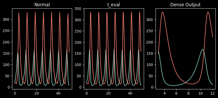
t_eval and dense output example
Read more about t_eval and dense output in “Documentation/Dense Output and t_eval.md”
[13]:
def cy_diffeq(dy, t, y):
    dy[0] = (1. - 0.01 * y[1]) * y[0]
    dy[1] = (0.02 * y[0] - 1.) * y[1]

from numba import njit
cy_diffeq = njit(cy_diffeq)

import numpy as np
from CyRK import pysolve_ivp

initial_conds = np.asarray((20., 20.), dtype=np.float64, order='C')
time_span = (0., 50.)
rtol = 1.0e-4
atol = 1.0e-5

result_normal = \
    pysolve_ivp(cy_diffeq, time_span, initial_conds, method="DOP853", rtol=rtol, atol=atol,
                pass_dy_as_arg=True)

print('Regular Shape: ', result_normal.y.shape)

# Use t_eval to provide more data points than the integrator used
t_eval = np.linspace(0., 50.0, 500)
result_t_eval = \
    pysolve_ivp(cy_diffeq, time_span, initial_conds, method="RK45", rtol=rtol, atol=atol,
                t_eval=t_eval,
                pass_dy_as_arg=True)

print('t_eval Shape: ', result_t_eval.y.shape)

# Or we could get the dense output and treat the result as a function
result_dense = \
    pysolve_ivp(cy_diffeq, time_span, initial_conds, method="RK45", rtol=rtol, atol=atol,
                dense_output=True,
                pass_dy_as_arg=True)

t_dense = np.linspace(3.0, 12.0, 250)
y_dense = result_dense(t_dense)
print('Dense Shape: ', y_dense.shape)

import matplotlib.pyplot as plt
fig, axes = plt.subplots(ncols=3, figsize=(10., 4.0))
axes[0].plot(result_normal.t, result_normal.y[0], c='C0')
axes[0].plot(result_normal.t, result_normal.y[1], c='C3')
axes[0].set(title='Normal')

axes[1].plot(result_t_eval.t, result_t_eval.y[0], c='C0')
axes[1].plot(result_t_eval.t, result_t_eval.y[1], c='C3')
axes[1].set(title='t_eval')

axes[2].plot(t_dense, y_dense[0], c='C0')
axes[2].plot(t_dense, y_dense[1], c='C3')
axes[2].set(title='Dense Output')

plt.show()
Regular Shape:  (2, 60)
t_eval Shape:  (2, 500)
Dense Shape:  (2, 250)
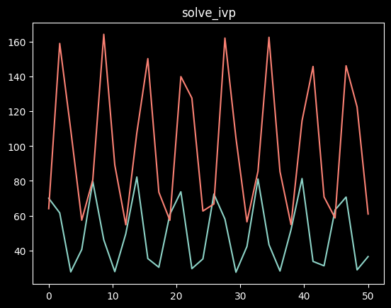
Backward Integration
[14]:
def diffeq(t, y):
    dy = np.empty_like(y)
    dy[0] = (1. - 0.01 * y[1]) * y[0]
    dy[1] = (0.02 * y[0] - 1.) * y[1]
    return dy

import numpy as np
from scipy.integrate import solve_ivp

initial_conds = np.asarray((70, 64.), dtype=np.float64, order='C')
# time_span = (0., 50.)
time_span = (50., 0.)
rtol = 1.0e-6
atol = 1.0e-8

t_eval = None
# t_eval = np.linspace(0.0, 50.0, 30)
# t_eval = np.linspace(50.0, 0.0, 30)


result = \
    solve_ivp(diffeq, time_span, initial_conds, method='RK45', rtol=rtol, atol=atol, t_eval=t_eval)

print("Was Integration was successful?", result.success)
print(result.message)
print("solve_ivp shape:", result.y.shape)
import matplotlib.pyplot as plt
fig, ax = plt.subplots()
ax.plot(result.t, result.y[0], c='C0')
ax.plot(result.t, result.y[1], c='C3')
ax.set(title='solve_ivp')
plt.show()


from CyRK import pysolve_ivp
result_cy = \
    pysolve_ivp(diffeq, time_span, initial_conds, method='RK45', rtol=rtol, atol=atol, t_eval=t_eval)

print("Was Integration was successful?", result.success)
print(result.message)
print("pysolve_ivp shape:", result_cy.y.shape)
import matplotlib.pyplot as plt
fig, ax = plt.subplots()
ax.plot(result_cy.t, result_cy.y[0], c='C0')
ax.plot(result_cy.t, result_cy.y[1], c='C3')
ax.set(title='pysolve_ivp')
plt.show()
Was Integration was successful? True
The solver successfully reached the end of the integration interval.
solve_ivp shape: (2, 173)
Was Integration was successful? True
The solver successfully reached the end of the integration interval.
pysolve_ivp shape: (2, 173)
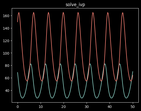
Backward Integration (with Dense)
[15]:
def diffeq(t, y):
dy = np.empty_like(y)
dy[0] = (1. - 0.01 * y[1]) * y[0]
dy[1] = (0.02 * y[0] - 1.) * y[1]
return dy
import numpy as np
from scipy.integrate import solve_ivp
initial_conds = np.asarray((70, 64.), dtype=np.float64, order='C')
time_span = (0., 50.)
# time_span = (50., 0.)
rtol = 1.0e-6
atol = 1.0e-8
t_eval = np.linspace(0.0, 50.0, 30)
# t_eval = np.linspace(50.0, 0.0, 30)
result = \
solve_ivp(diffeq, time_span, initial_conds, method='RK45', rtol=rtol, atol=atol, dense_output=True)
print("Was Integration was successful?", result.success)
print(result.message)
print("solve_ivp shape:", result.y.shape)
import matplotlib.pyplot as plt
fig, ax = plt.subplots()
sci_dense = result.sol(t_eval)
ax.plot(t_eval, sci_dense[0], c='C0')
ax.plot(t_eval, sci_dense[1], c='C3')
ax.set(title='solve_ivp')
plt.show()
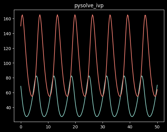
from CyRK import pysolve_ivp
result_cy = \
pysolve_ivp(diffeq, time_span, initial_conds, method='RK45', rtol=rtol, atol=atol, dense_output=True)
print("Was Integration was successful?", result.success)
print(result.message)
print("pysolve_ivp shape:", result_cy.y.shape)
import matplotlib.pyplot as plt
fig, ax = plt.subplots()
pysolve_dense = result_cy(t_eval)
ax.plot(t_eval, pysolve_dense[0], c='C0')
ax.plot(t_eval, pysolve_dense[1], c='C3')
ax.set(title='pysolve_ivp')
plt.show()
print(np.allclose(pysolve_dense, sci_dense))
Was Integration was successful? True
The solver successfully reached the end of the integration interval.
solve_ivp shape: (2, 175)
Was Integration was successful? True
The solver successfully reached the end of the integration interval.
pysolve_ivp shape: (2, 175)
True
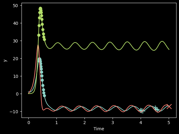
Events
Events with SciPy
[16]:
import numpy as np
from scipy.integrate import solve_ivp
import matplotlib.pyplot as plt

# Example with SciPy
def event_func_1(t, y, a, b, c):

    # Check if t greater than or equal to 5.0
    if t >= 5.0:
        return 0.0
    else:
        return 1.0

def event_func_2(t, y, a, b, c):

    # Check y values.
    # In the time span [0,10]:
    #    y_0  starts at 1, spikes then goes below zero and oscillates with a min below -10. Have this return if y_0 < -10
    if y[0] < -10.0:
        return 0.0
    elif y[2] > 30.0:
        return 0.0
    else:
        return 1.0


def event_func_3(t, y, a, b, c):

    # We won't actually use the args but lets just check they are correct.
    args_correct = False
    if a == 10.0 and b == 28.0 and c == 8.0 / 3.0:
        args_correct = True

    # Then return events if args are correct and t greater than 4 (only every .5)
    if args_correct and t >= 4:
        if t <= 4.1:
            return 0.0
        elif t >= 4.5 and t <= 4.6:
            return 0.0
        elif t >= 5.0 and t <= 5.1:
            return 0.0
        elif t >= 5.5 and t <= 5.6:
            return 0.0
        elif t >= 6.0 and t <= 6.1:
            return 0.0
        else:
            return 1.0
    else:
        return 1.0

def lorenz_diffeq(t, y, a, b, c):
    # Unpack y
    y0 = y[0]
    y1 = y[1]
    y2 = y[2]

    dy = np.empty(3, dtype=np.float64)

    dy[0] = a * (y1 - y0)
    dy[1] = y0 * (b - y2) - y1
    dy[2] = y0 * y1 - c * y2
    return dy

def run_scipy_with_events(terminate = False):

    event_func_1.direction = 0
    event_func_1.terminal = 10000
    if terminate:
        event_func_1.terminal = 1
    event_func_2.direction = 0
    event_func_2.terminal = 10000
    event_func_3.direction = 0
    event_func_3.terminal = 10000


    time_span = (0.0, 10.0)
    y0 = np.asarray([1.0, 0.0, 0.0])
    args = (10.0, 28.0, 8.0/3.0)
    solution = solve_ivp(lorenz_diffeq, time_span, y0, method="RK45",
                         args=args, rtol=1.0e-6, atol=1.0e-6, t_eval=None, dense_output=False,
                         events=(event_func_1, event_func_2, event_func_3))

    return solution
[17]:
# SciPy Times
#  terminate off: 23.6ms; 23.7ms; 23.8ms
#  terminate on:  10.5ms; 10.3ms; 10.4ms

terminate = True
solution = run_scipy_with_events(terminate)

%timeit run_scipy_with_events(terminate)

fig, ax = plt.subplots()
ax.plot(solution.t, solution.y[0], label='y0', c='C0')
ax.plot(solution.t, solution.y[1], label='y1', c='C3')
ax.plot(solution.t, solution.y[2], label='y2', c='C6')
# Event 1 will be dots.
# Event 2 will be X's
# Event 3 will be +'s
ax.scatter(solution.t_events[1], solution.y_events[1][:, 0], c='C0', marker='o')
ax.scatter(solution.t_events[0], solution.y_events[0][:, 1], c='C3', marker='x', s=120)
ax.scatter(solution.t_events[1], solution.y_events[1][:, 2], c='C6', marker='o')
ax.scatter(solution.t_events[2], solution.y_events[2][:, 0], c='C0', marker='+', s=120)
ax.set(xlabel='Time', ylabel='y')
plt.show()
5.71 ms ± 70.5 μs per loop (mean ± std. dev. of 7 runs, 100 loops each)
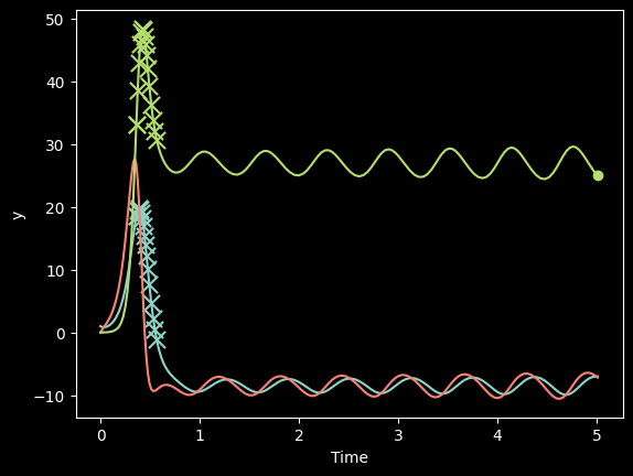
Events with pysolve_ivp
[18]:
import numpy as np
from CyRK import pysolve_ivp
import matplotlib.pyplot as plt
from numba import njit

# Example with SciPy
@njit
def event_func_1(t, y, a, b, c):

    # Check if t greater than or equal to 5.0
    if t >= 5.0:
        return 0.0
    else:
        return 1.0

@njit
def event_func_2(t, y, a, b, c):

    # Check y values.
    # In the time span [0,10]:
    #    y_0  starts at 1, spikes then goes below zero and oscillates with a min below -10. Have this return if y_0 < -10
    if y[0] < -10.0:
        return 0.0
    elif y[2] > 30.0:
        return 0.0
    else:
        return 1.0

@njit
def event_func_3(t, y, a, b, c):

    # We won't actually use the args but lets just check they are correct.
    args_correct = False
    if a == 10.0 and b == 28.0 and c == 8.0 / 3.0:
        args_correct = True

    # Then return events if args are correct and t greater than 8
    if args_correct:
        return 0.0
    else:
        return 1.0

@njit
def lorenz_diffeq(dy, t, y, a, b, c):
    # Unpack y
    y0 = y[0]
    y1 = y[1]
    y2 = y[2]

    dy[0] = a * (y1 - y0)
    dy[1] = y0 * (b - y2) - y1
    dy[2] = y0 * y1 - c * y2

def run_pysove_with_events(terminate = False):

    event_func_1.direction = 0
    event_func_1.terminal = 10000
    if terminate:
        event_func_1.terminal = 1
    event_func_2.direction = 0
    event_func_2.terminal = 10000
    event_func_3.direction = 0
    event_func_3.terminal = 10000


    time_span = (0.0, 10.0)
    y0 = np.asarray([1.0, 0.0, 0.0])
    args = (10.0, 28.0, 8.0/3.0)
    solution = pysolve_ivp(lorenz_diffeq, time_span, y0, method="RK45",
                           args=args, rtol=1.0e-6, atol=1.0e-6, t_eval=None, dense_output=False, pass_dy_as_arg=True,
                           events=(event_func_1, event_func_2, event_func_3))

    return solution
[19]:
# PySolver Times
#   CyRK v0.16.0 (njit-off)
#     terminate off: 1.20ms; 1.22ms; 1.73ms
#     terminate on:  612us; 631us; 620us
#   CyRK v0.16.0 (njit-on)
#     terminate off: 642us; 634us; 648us
#     terminate on:  314us; 310us; 314us


terminate = True
solution = run_pysove_with_events(terminate)

%timeit run_pysove_with_events(terminate)

fig, ax = plt.subplots()
ax.plot(solution.t, solution.y[0], label='y0', c='C0')
ax.plot(solution.t, solution.y[1], label='y1', c='C3')
ax.plot(solution.t, solution.y[2], label='y2', c='C6')
# Event 1 will be dots.
ax.scatter(solution.t_events[0], solution.y_events[0][2, :], c='C6', marker='o')
# Event 2 will be X's
ax.scatter(solution.t_events[1], solution.y_events[1][0, :], c='C0', marker='x', s=120)
ax.scatter(solution.t_events[1], solution.y_events[1][2, :], c='C6', marker='x', s=120)
# Event 3 we won't plot because it should be every point.
ax.set(xlabel='Time', ylabel='y')
plt.show()
296 μs ± 5.15 μs per loop (mean ± std. dev. of 7 runs, 1,000 loops each)
Parallelizing pysolve_ivp
Example of how to parallelize pysolve_ivp using Python’s multiprocessing package.
To ensure that the workers don’t try to read the entire Jupyter Notebook thread we will wrote helper functions to a separate file found in this directory called “pysolve_parallel.py”
[20]:
import multiprocessing
import numpy as np
# Import the functions we just wrote to disk
import pysolve_parallel
import time

def run_notebook_parallel():
    num_simulations = 500
    base_y0 = np.array([10.0, 5.0])

    # Create the task list
    tasks = []
    for i in range(num_simulations):
        # Note: We pass 'pysolve_parallel.my_diffeq', not a local function
        task_params = (
            pysolve_parallel.my_diffeq,
            (0.0, 200.0),
            base_y0,
            (1.5, 1.0, 3.0, 1.0),
            1e-5,
            1e-8
        )
        tasks.append(task_params)

    # Use 'with' context manager to ensure pool closes
    # We use pysolve_parallel.solve_worker so the parallel process can find it
    for procs in range(1, multiprocessing.cpu_count()):
        print(f"Working with {procs} processes...")
        t0 = time.perf_counter_ns()/1.0e9
        with multiprocessing.Pool(processes=procs) as pool:
            results = pool.map(pysolve_parallel.solve_worker, tasks)
        t1 = time.perf_counter_ns()/1.0e9
        print(f"\tFinished in {(t1-t0):0.2f} s.\n")

if __name__ == "__main__":
    print("Triggering parallelized cell...")
    run_notebook_parallel()
Triggering parallelized cell...
Working with 1 processes...
        Finished in 6.15 s.

Working with 2 processes...
        Finished in 3.27 s.

Working with 3 processes...
        Finished in 2.35 s.

Working with 4 processes...
        Finished in 1.87 s.

Working with 5 processes...
        Finished in 1.58 s.

Working with 6 processes...
        Finished in 1.48 s.

Working with 7 processes...
        Finished in 1.35 s.

Working with 8 processes...
        Finished in 1.25 s.

Working with 9 processes...
        Finished in 1.22 s.

Working with 10 processes...
        Finished in 1.20 s.

Working with 11 processes...
        Finished in 1.20 s.

Working with 12 processes...
        Finished in 1.26 s.

Working with 13 processes...
        Finished in 1.22 s.

Working with 14 processes...
        Finished in 1.19 s.

Working with 15 processes...
        Finished in 1.18 s.